
KQL for Adults: Writing Queries That Don't Lie to You
You ran the query. Got results. Moved on. But did you actually ask the question you thought you asked?
KQL is easy enough to start with that most people never really stop to question the mental model they brought to it. The pipe syntax feels familiar. Filtering reads almost like natural language. Results come back fast. So teams start writing alert rules, dashboards, and detection queries before they’ve developed the instincts to know when those results are quietly wrong.
The language won’t tell you. KQL doesn’t warn you that your join just scanned two years of data. It won’t flag that your string filter is doing a full column scan instead of an index lookup, or that the events your alert is supposed to catch are falling into a gap your time window doesn’t cover. It just returns results. Confidently. Every time.
What follows are three failure modes, roughly in order of how obviously they manifest. The first is visible if you know what to look for. The second hides in query structure. The third is almost invisible — and it’s the one that matters most if you’re running detections.
The Operator You’re Using Means Something Different Than You Think
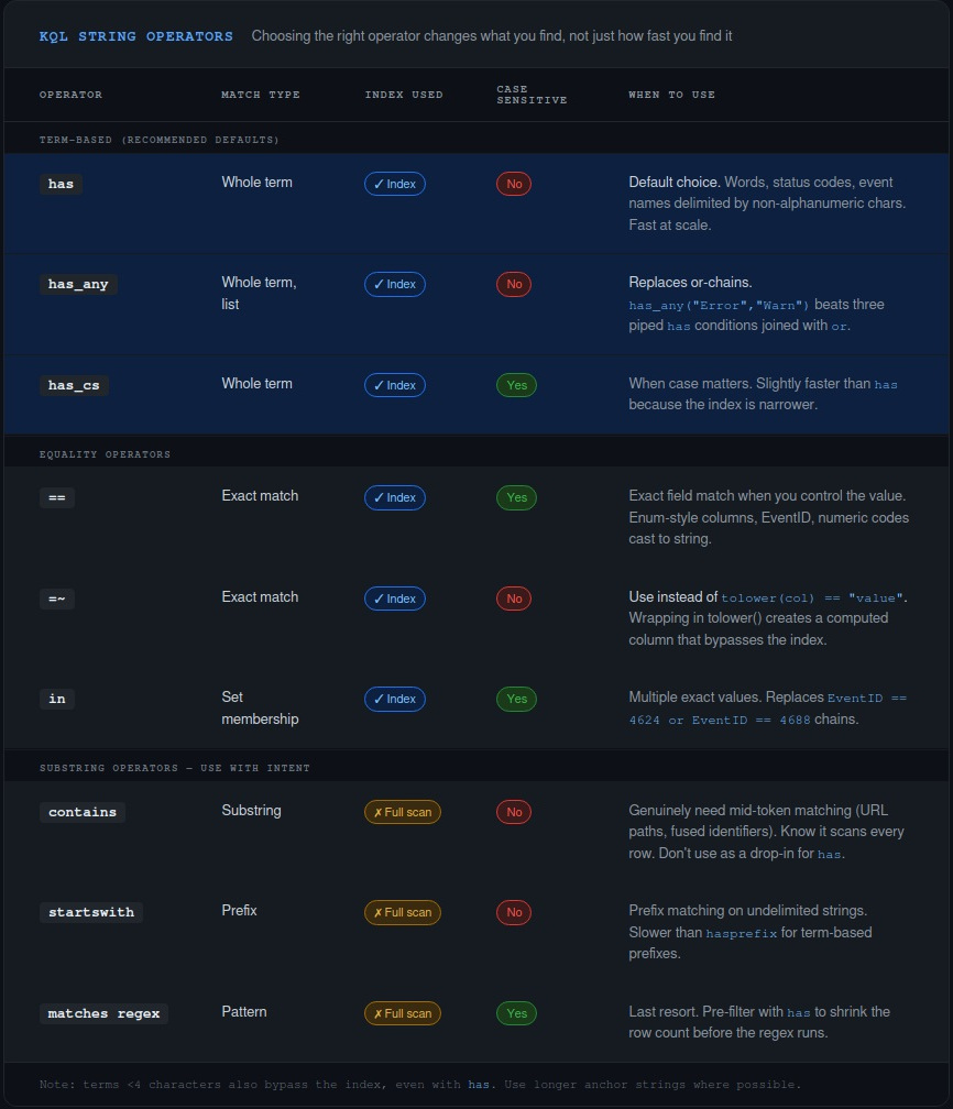
Most people come to KQL from SQL, grep, or Splunk. All of those transfer poorly because KQL’s string matching is term-based, not character-based. Azure Data Explorer indexes string columns by breaking values into tokens — maximal sequences of alphanumeric characters separated by non-alphanumeric delimiters. The has family of operators uses that index. contains does not.
This isn’t just a performance difference. They can return different results.
"KustoExplorerQueryRun" has "Explorer"     // returns false
"KustoExplorerQueryRun" contains "Explorer" // returns true
KustoExplorerQueryRun is one term. There’s no delimiter between Kusto, Explorer, and QueryRun — they’re fused into a single alphanumeric sequence. has looks for whole terms and can’t find Explorer inside a larger one. contains does a substring scan and finds it immediately.
So when you write | where Message contains "Error" because you want to find error events, you might be getting more than you bargained for — matching words like ErrorCode, HandleErrors, isErrored — and you’re paying for a full table scan to do it. If you mean “find records where the word Error appears as a complete term,” has is what you want. It’s also faster, because it uses the index.
The practical operator guide:
has— whole term match, case-insensitive, uses the index. Default choice for filtering on words, status strings, event names.contains— substring match, full scan. Use it when you genuinely need to find a pattern inside a larger token (URL paths, identifiers). Know it’s expensive.=~— case-insensitive equality. Use this instead oftolower(col) == "value". Wrapping a column intolower()creates a computed value the engine can’t index.has_any(list)— equivalent tohasacross multiple values. Much better than chainingorconditions.
That last point catches people who know about has but haven’t thought about the multi-value case. An or chain evaluates each condition sequentially. has_any() is a set membership check and significantly more efficient when you’re matching against more than a couple of values.
// Slower — sequential evaluation
| where AppDisplayName has "Teams"
    or AppDisplayName has "Outlook"
    or AppDisplayName has "SharePoint"

// Faster — set-based check
| where AppDisplayName has_any ("Teams", "Outlook", "SharePoint")
Same result. Different cost at scale.
Your Time Window Isn’t What You Think It Is
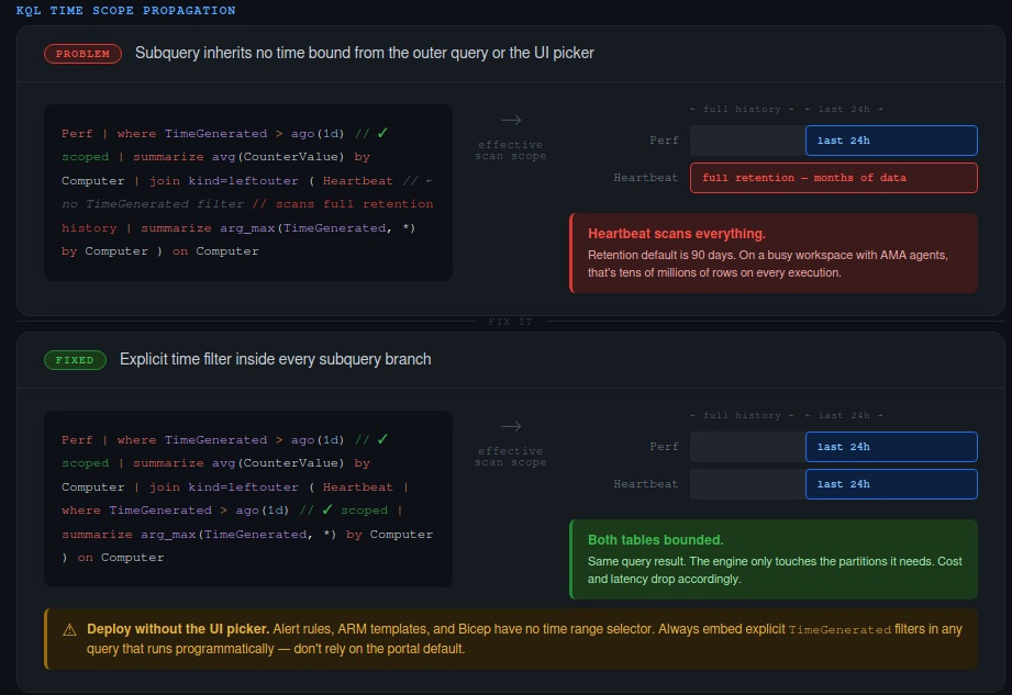
Time is the most common filter in any log query. It’s also the most commonly misapplied — not because people write it wrong, but because the structure of the query creates gaps they don’t see.
The Log Analytics UI time picker applies to the outer query. Subqueries in join and union branches don’t inherit it. If you have a join and the inner query has no TimeGenerated filter of its own, it will scan the full retention history of that table. Silently. Every time the query runs.
Here’s what it looks like:
Perf
| where TimeGenerated > ago(1d)
| summarize avg(CounterValue) by Computer, CounterName
| join kind=leftouter (
    Heartbeat
    // No time filter here — scans all of Heartbeat's history
    | summarize arg_max(TimeGenerated, *) by Computer
) on Computer
The outer query is nicely bounded to the last 24 hours. The Heartbeat subquery isn’t bounded at all. Depending on your retention policy, that could mean months of data being scanned on every execution. If this query backs a dashboard that refreshes every few minutes, the cost accumulates quickly.
The fix is explicit — propagate the time bound into every subquery:
Perf
| where TimeGenerated > ago(1d)
| summarize avg(CounterValue) by Computer, CounterName
| join kind=leftouter (
    Heartbeat
    | where TimeGenerated > ago(1d)  // scoped
    | summarize arg_max(TimeGenerated, *) by Computer
) on Computer
The same problem shows up with union. If you apply a TimeGenerated filter after the union rather than inside each branch, both tables get fully scanned before the filter applies. Apply the time filter inside each branch, not as a post-union where clause.
There’s a related trap that affects anyone deploying queries programmatically. You test a query in the portal with the time picker set to “Last 24 hours.” It looks right. You export the query to an ARM template or Bicep file for your alert rule. The picker doesn’t exist in that context. If your query doesn’t have an embedded TimeGenerated filter, it’s now running against unbounded data on every evaluation cycle. This happens more than it should.
The other structural inefficiency worth knowing: filtering on a column you’ve created with extend forces the engine to evaluate the expression for every row before it can filter. Filter on physical columns first, extend afterwards.
// Expensive — filter on computed column
Syslog
| extend Msg = strcat("Syslog: ", SyslogMessage)
| where Msg has "Error"

// Better — filter on the source column
Syslog
| where SyslogMessage has "Error"
And if you find yourself joining the same table to itself to get two different counts, reach for countif instead:
// Two scans
SecurityEvent
| where EventID == 4624
| summarize LoginCount = count() by Account
| join (
    SecurityEvent
    | where EventID == 4688
    | summarize ExecutionCount = count() by Account
) on Account

// One scan
SecurityEvent
| where EventID in (4624, 4688)
| summarize
    LoginCount     = countif(EventID == 4624),
    ExecutionCount = countif(EventID == 4688)
  by Account
Same output. The second scans the table once.
The Data Isn’t There When You Think It Is
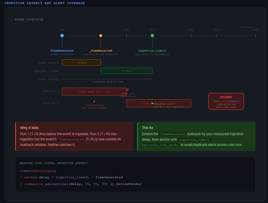
This is the one most people don’t know about, and it matters most for anyone running scheduled detection rules.
There are three timestamps associated with every log record in Azure Monitor, and they mean different things:
TimeGenerated— when the event was created at the source. This is the column partitioned for querying, what the time picker filters on, and what you use in almost every investigation._TimeReceived— when the log reached the Azure Monitor ingestion endpoint.ingestion_time()— when the record became queryable in your workspace.
The gap between TimeGenerated and ingestion_time() is ingestion latency. It’s never zero. For many sources it’s a few seconds or minutes. For some third-party connectors, the 99th percentile latency exceeds 55 minutes.
Here’s why that matters for detection. Say you have a Sentinel analytics rule that runs every five minutes with a five-minute lookback. An event is generated at T+0. It doesn’t get ingested until T+7. The rule ran at T+5 and T+10. At T+5, the event wasn’t in the workspace yet. At T+10, its TimeGenerated timestamp (T+0) is outside the five-minute lookback window. Neither run catches it. The event sits in your workspace, permanently undetected by that rule.
Microsoft Sentinel has a built-in five-minute buffer — rules actually look back a little further than configured. But for sources with tail latency measured in tens of minutes, that buffer isn’t enough.
The first thing to do is measure your actual ingestion delay:
CommonSecurityLog
| extend delay = ingestion_time() - TimeGenerated
| summarize percentiles(delay, 50, 95, 99) by DeviceVendor
Run this against your real data. The p99 number is what you care about for coverage guarantees. Don’t guess — the answer will vary significantly by source.
Once you know the delay for a given source, you can account for it in your detection query:
let ingestion_delay = 4min;
let rule_look_back  = 5min;
CommonSecurityLog
| where TimeGenerated >= ago(ingestion_delay + rule_look_back)
| where ingestion_time() > ago(rule_look_back)
The first where extends the TimeGenerated lookback window to catch late-arriving records. The second anchors the rule to only alert on records ingested in the current window. Without that ingestion_time() anchor, extending the lookback causes duplicate alerts because the same event will be found by multiple consecutive rule runs.
Write It Like It Matters
A query backing an alert rule is evidence. It’ll be referenced in a post-incident review, questioned in a FinOps discussion, or audited for compliance. “It returns results” isn’t the same as “it’s correct.”
The practical checklist is short: use has when you mean whole-word matching; scope every subquery’s time bounds explicitly; deploy embedded TimeGenerated filters rather than relying on the portal picker; and for any detection rule, measure your source’s ingestion latency before you trust the coverage.
The more honest question to ask yourself when you write a query is whether you could defend it if the results were challenged. Not “does it look right?” but “can you explain what it’s actually asking, why it’s bounded the way it is, and what it might be missing?”
Most KQL that runs in production can’t answer that. Yours should be able to.
What’s the worst silent failure you’ve found in a query that had been running in production for months? The ingestion latency one tends to produce some interesting stories.
